|
|
| source code: | CSEE-source.zip |
| executable: | CSEE.zip |
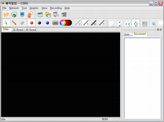
In Slideshow view, you can load PPT/PDF or image files into CSEE, and start a lecture.
|
|
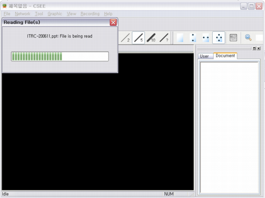
Click File-Open... to load a file, there will be a progress dialog popping up. (Figure 2)
|
|
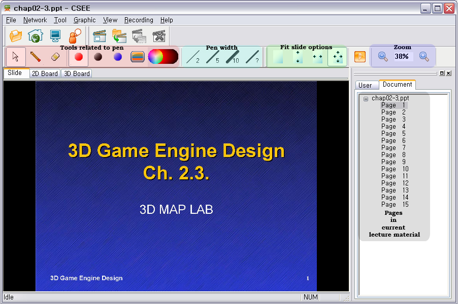
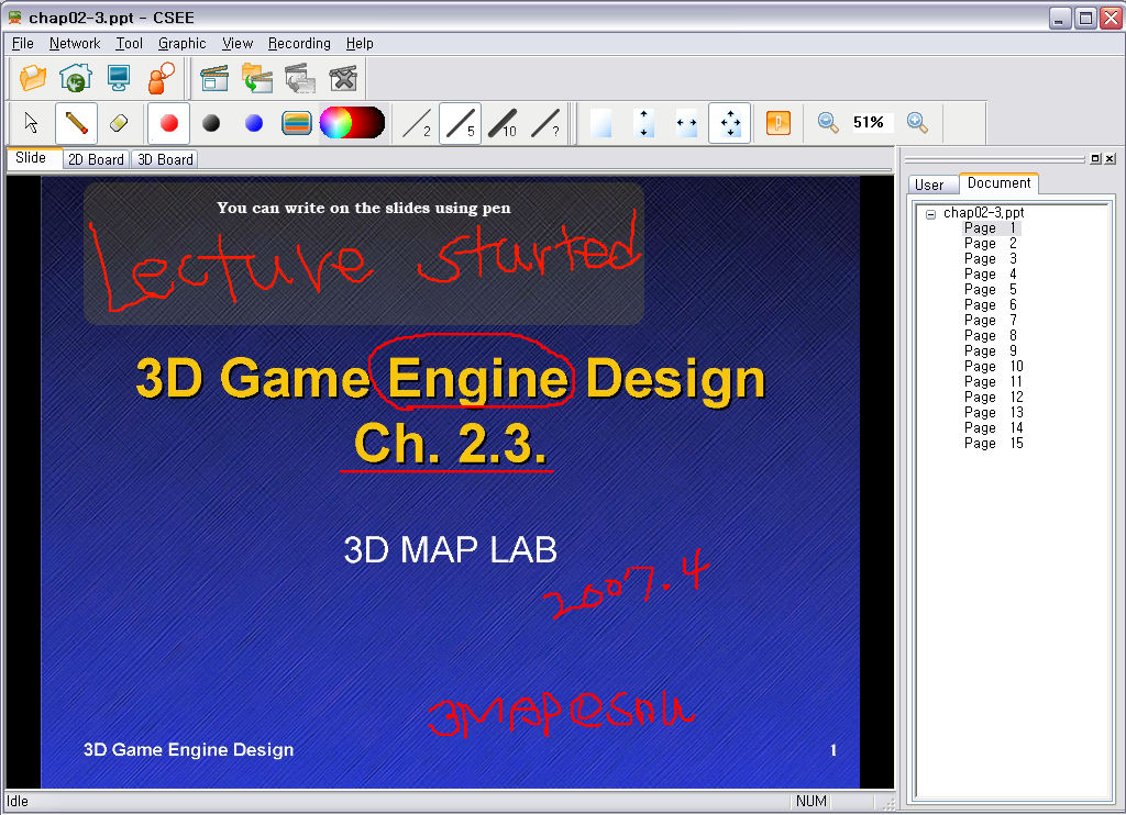
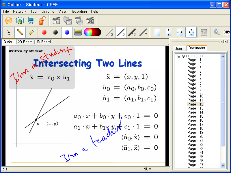
Once the file has been loaded, the lecture file will appear on the screen. Now we can draw on the slides using Tablet pen or move to other pages.
|
|
To start distance lecture between an instructor and students, select Network-Connect..., and a connect dialog will show up. The instructor sets his/her computer as a server, and students connect to the instructors computer to participate in the lecture. In the current implementation, the instructor needs an IP address. The system automatically sets an IP address from network configuration. The instructor needs to set a port number and press Create button. The students need to type in the instructors IP address and press Connect button to participate in the lecture. Once the connection between the instructor and students is established, their activities are synchronized.
|
|
|
|
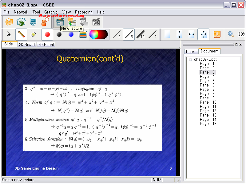
You can record your own lecture using CSEE.
|
|
Lecture recording toolbar is similar to those of a cassette player. You can start recording by pressing a button with small red circle. Voice, scribbles, transitions between views on CSEE will be recorded during the lecture recording.
|
|
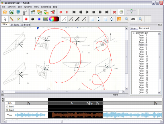
When you select View-Recording
Window, you can edit a recorded file.
|
|
(1) Conic section drawing by free-hand sketch and interactive editing.
-
Parabola, Ellipse, Hyperbola
(2) Conic section drawing by entering coefficients.
(3) Fitting free-hand sketch to a conic section by the SVD method.
(4) Polynomial function drawing (up to quartic).
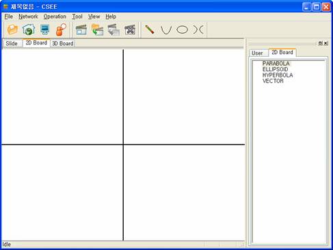
(1) Conic primitive drawing and editing.
Step 1.
Select ![]()
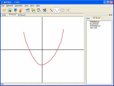
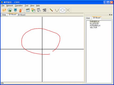
Step 2. Sketch a parabola in one stroke as follows.
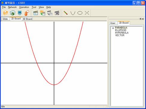
Step 3. CSEE will automatically change
the above sketch to a fitted parabola.
You can also
see the equation of this curve on the right tab view.
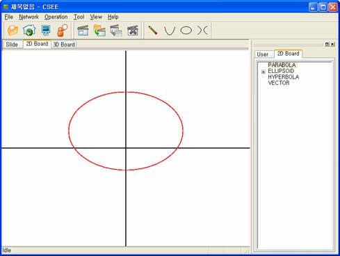
Step 4.
Drawing an ellipse.
Select ellipse tool ![]()
Sketch an
ellipse within one stroke.
A fitted ellipse of the above sketch will show up as follows.
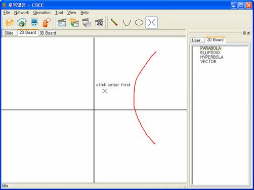
Step 5.
Drawing a hyperbola.
Select the
hyperbola tool ![]()
First, click the center position of the hyperbola.
Then sketch a half of the hyperbola (right, left, upper or lower half).
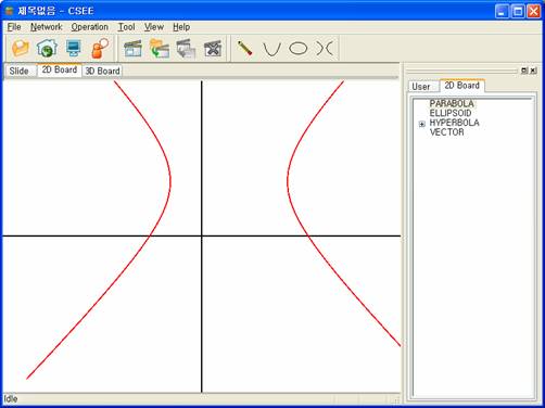
A fitted hyperbola will show up as follows.
Step 6. How
to edit
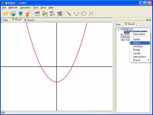
Find the
equation of the object on the right side and select it, then the
selected object can be edited.
In the editing
mode, the object will change its color and its control points will show up.
If you
want to drag one of the control points,
you have to select Operation
> drag to modify (discrete) on menu and drag a central point.
Changes in
control points produce different effects according to the object type and the role of each
control point of that type.
- Parabola -
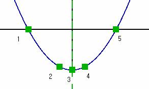
1, 5, 2, 4 : Control the width of parabola.
3 : Control the position of parabola (center
position)
- Ellipse -
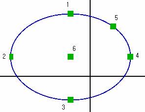
1, 3 :
Control the height of ellipse.
2, 4 : Control the width of ellipse.
5 : Control the height and width of ellipse
simultaneously.
6 : Control the center point of ellipse.
- Hyperbola -
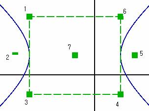
1, 3, 4, 6 : Control asymptotic curves of hyperbola.
2, 5 : Control focus distance of hyperbola.
7 : Control center position of hyperbola.
You can draw a general conic section by entering coefficients of each
term in a dialog box.
First select Operation > Conic Drawing on menu.
Then enter coefficients into edit boxes of each term, and set a bounding box in
which the conic section will be drawn.
You can select the number of samples of the Marching Cube
algorithm.
Then push the (re)Draw button to draw it on the canvas.
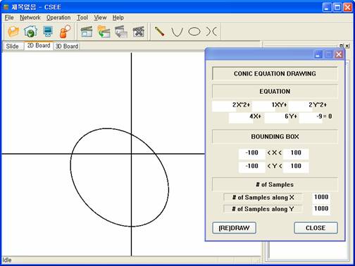
This figure shows 2x^2 + xy + 2y^2 + 4x + 6y
9 = 0.
Your freehand sketch can be fitted into a general
conic section by CSEE.
Select Operation > Semi-Automatic Conic Fitting on menu.
Sketch any shape you want, then a conic equation (fitted by the minimum square
solution of the SVD method) will show up.
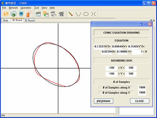
This figure shows a freehand sketch (red curve) and a fitted conic section (black
ellipse) and its equation on the right dialog.
You can draw a graph of polynomial functions up to quartic polynomial.
Select Operation > f(x) Function Drawing.
Enter coefficients and domain range and line segment sampling intervals, then push the draw button.
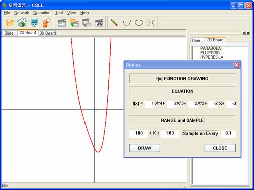
Example screen of f(x) Function Drawing operation.
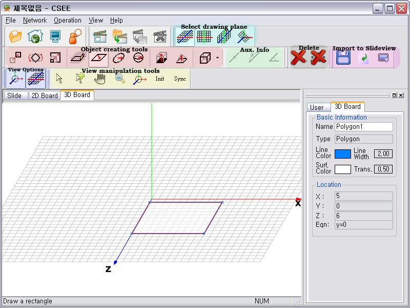
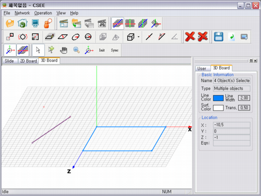
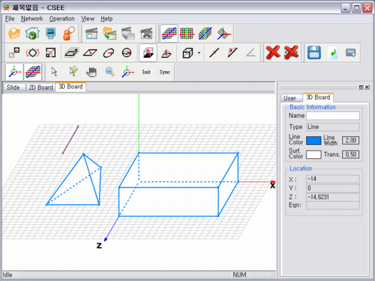
You can create 3D objects using toolbar. For a free drawing, the default drawing plane is the XZ plane. You can draw a point and extrude it to a line, extrude a line to a plane, and extrude a plane to an object. There are also predefined primitives.
|
|
|
|
|
|
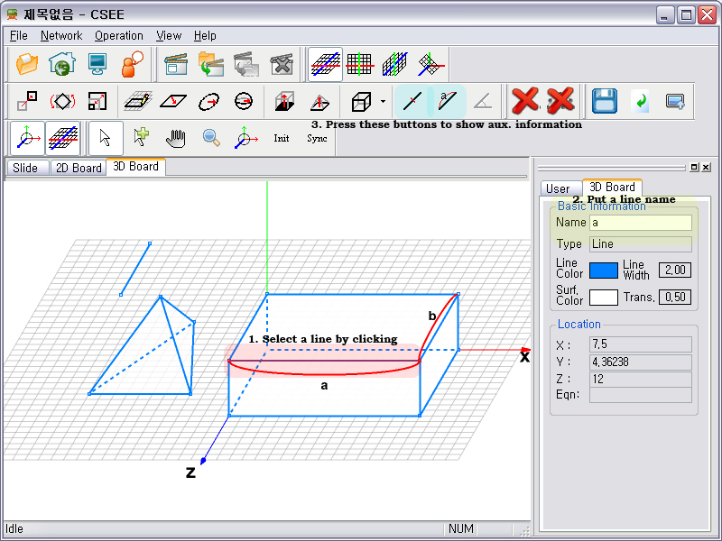
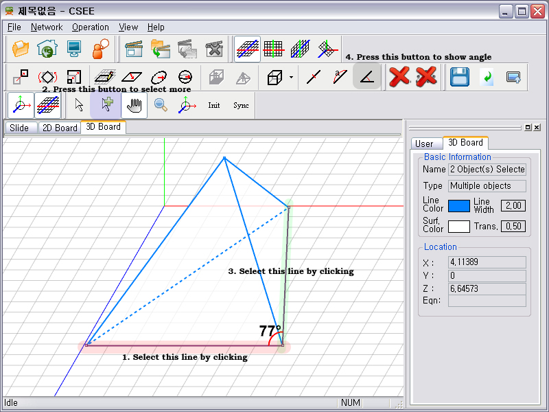
You can select an object by clicking. Every time you click on the window, CSEE decides which one to select. If there are more than one object, you can select one by clicking twice or more on the same point. You can also put auxiliary information.
|
|
|
|
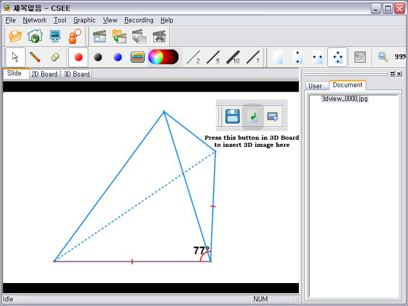
Objects created in 3D Board can be imported into Slideview.
|
|